Optimized Real Time N-Body Simulation - Part 1 Brute Force Method
N-body Shenanigans (Writing In Progress)#
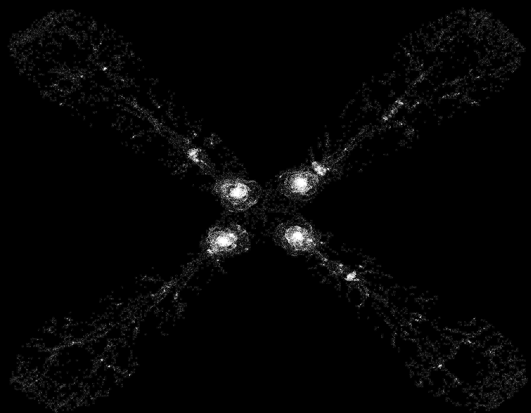
We’ve all seen those cool simulations colliding or a black hole sucking everything up. I find them pretty cool to look at. Wondering how every particle gets simulated made me even more interested and also broke my brain. Eager to satisfy this curiosity and not let my brain cells die in vain, I put myself through the long, arduous journey of trying to make my own. Of course the fruits of this quest blessed the world with the fantastically written (you have been warned) N-body simulation optimized with parallelized quad-tree constructions using morton order sorting capable of running 200,000 independent particles in real-time!
If you have no idea what either of those words mean, neither did I a couple weeks ago. But do not worry, after reading this we will both be super-experts in optimizing N-body simulations.
Simple Pair Interactions#
The simulation initially employed the Brute Force N-body Method, which is a direct approach whereby the gravitational attraction between each pair of particles is calculated. At a given time step, the net force acting on a particle is computed, and its position and acceleration are updated using Euler’s Method for numerical integration as follows:
$$ \mathbf{a}_i^n = -G \sum_{\substack{j=1 \\ j \neq i}}^{N} m_j \frac{\mathbf{r}_j^n - \mathbf{r}_i^n}{\left( \| \mathbf{r}_j^n - \mathbf{r}_i^n \|^2 + \epsilon^2 \right)^{3/2}} \ $$Woah, scary physics equation! What does it mean? Well it pretty much shows the acceleration a particle experiences is the cumulative effect of the gravitational force from all other particles.
We update our velocity and position like below:
$$ \begin{align*} \textbf{Velocity update :} \quad & \mathbf{v}_i^{n+1} = \mathbf{v}_i^n + \mathbf{a}_i^n \Delta t \\ \textbf{Position update :} \quad & \mathbf{r}_i^{n+1} = \mathbf{r}_i^n + \mathbf{v}_i^n \Delta t \end{align*}$$- \( G \): Gravitational constant
- \( \mathbf{r}_i^n \): Position of body \( i \) at step \( n \)
- \( \mathbf{v}_i^n \): Velocity of body \( i \) at step \( n \)
- \( \epsilon \): Softening length (avoids singularities when \( r_{ij} \to 0 \))
- \( \Delta t \): Time step size
The softening factor \( \epsilon\) is super important, because since we are not gonna implement collisions, our particles theoretically will be on top of each other, and thus the distance between them will be so infinitesimally small that the force will explode to such an incomprehensibly high number that our poor particle will zip out of existence.
Here’s the code for calculating the acceleration experienced by a given body
std::vector<float> computeAcceleration(const Body& obj1, const Body& obj2, float s_gamma, float s_soft) {
    std::vector<float> acc(2, 0.0f);

    //Return zero acceleration if the objects are the same
    if (&obj1 == &obj2) {
        return acc;
    }

    float x1 = obj1.position[0];
    float y1 = obj1.position[1];
    float x2 = obj2.position[0];
    float y2 = obj2.position[1];

    float m1 = obj1.mass;
    float m2 = obj2.mass;

    //Compute softened distance to avoid singularity
    double r = sqrt((x1 - x2) * (x1 - x2) + (y1 - y2) * (y1 - y2) + s_soft);

    if (r > 0) {
        double k = s_gamma * m2 / (r * r);
        acc[0] += k * (x2 - x1);
        acc[1] += k * (y2 - y1);
    } else {
        acc[0] = acc[1] = 0;
    }

    return acc;
}
Our Euler step method is implemented for the object class as seen below:
Object::Object()
    : position({0.0f, 0.0f}), velocity({0.0f, 0.0f}), radius(1.0f), mass(1.0f){}

Object::Object(std::array<float, 2> position, std::array<float, 2> velocity, float radius, float mass)
    : position(position), velocity(velocity), radius(radius), mass(mass){}

void Object::accelerate(float x, float y, float dt){
    velocity[0] += x * dt;
    velocity[1] += y * dt;
}

void Object::updatePos(float dt){
    position[0] += velocity[0] * dt;
    position[1] += velocity[1] * dt;
}
The accelerate function updates our velocity by taking acceleration in the x and y directions. After that, we call our updatePos function which uses our updated velocities to compute the new position.
TA DA! Lovely, lovely N-body simulation that you can show your friends! But wait, there is a catch to this simulation.
Performance of Brute Force Simulation#
I’m going to be testing this SOT simulation on an increasing number of bodies to see how the performance scales.
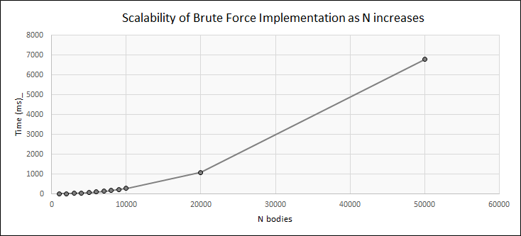 This brute-force implementation of an N-body simulation gets mad when we increase the number of bodies and slows down significantly. It takes almost 7 seconds to render a single frame at 50000 bodies, far away from the 200,000 body real-time simulation I promised you. Don’t leave yet! We have haven’t even reached the tip of the iceberg when it comes to optimizing this simulation. The next part of this story will be journey of beautiful spatial partitioning and dopamine inducing N-body interactions. Stay tuned!